In today's world, there might only be a few people who aren't aware of what “Machine Learning” and “Artificial Intelligence” are. It's the new craze. In fact, as per Linkedin, artificial intelligence specialists and data scientists are two of the top three emerging jobs in the United States.
It can often be difficult to understand how different machine learning models work, and the difference between them. To fathom this, we’ve made a list of the top ten most common and useful algorithms for those starting out. You’ll learn the fundamental differences between the various kinds of machine learning models and figure out how to pick the right one for your problem at hand.
Machine Learning can be defined as a method of data analysis that automates analytical model building - where the models learn from data, identifies, and predicts patterns - while making decisions with minimal human intervention.
There are three broad categories under which the algorithms fall under:
1. Supervised Algorithms: data is labeled and the algorithm learns to predict the output from input data
2. Unsupervised Algorithms: data is unlabeled and the algorithm learns the inherent structure from the input data
3. Reinforcement Algorithms: where an agent learns by interacting with an environment, taking actions, and learning from the consequences.
Of course the success of a model is highly dependent on the quality of the data. Poor data is the enemy of machine learning. If you have garbage data coming in, you’ll more than likely have garbage results on the other end. This is one of the reasons why data scientists often spend more than half of their time cleansing datasets before training and running models.
You may also like our beginner's guide to Machine Learning
Each model has its own strengths and weaknesses, which means it’s important to understand the scenario you’re trying to solve for and picking a few that fit your question.

1. Linear Regression
Linear regressions are models that show the relationships between an independent and dependent variable. It has two main objectives:
-
To establish if there is a relationship between two variables
-
To forecast or predict new observations
A positive relationship exists if one variable increases and the other variable increases as well. Linear Regressions are great to test if a relationship exists, and then use what you know about an existing relationship to forecast unobserved values.
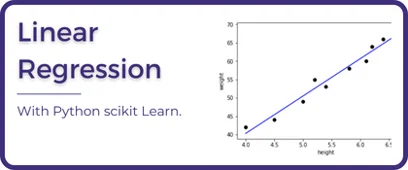
It begins with the name linear because we use a linear equation which appears as a straight line when plotted as seen below.
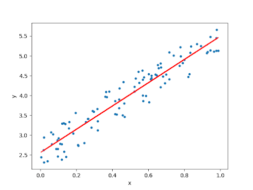
[Figure 1]
A logistic regression can be calculated as: Y = A + Bx
The goal of linear regressions is to fit a line that is nearest to all of the data points. Because the plotted output of this model is always in a straight line and never curved, it is very simple to perform and easy to understand.
Remember however that with its simplicity, it has its limits. Linear Regressions aren't applicable everywhere.
2. Logistic Regression
Rather than using continuous variables in linear regression, logistic regression models are based on discrete values. It is best suited for making predictions using binary classifications. For example, whether students passed or failed an exam (Yes or No).
Logistic regressions seek to model the probability of an event occurring depending on the values of the independent variables (either categorical or numerical). It can also be used to estimate the probability that an event occurs for a randomly selected observation and predict the effect of a series of variables on a binary response variable.
Unlike linear regression, logistic regressions transform outputs using the logistic sigmoid function to return a probability value which can then be mapped to two or more discrete classes.
Instead of fitting a line to the data, logistic regression fits an S-shaped logistic function to classify the data points into one of the two binary values.
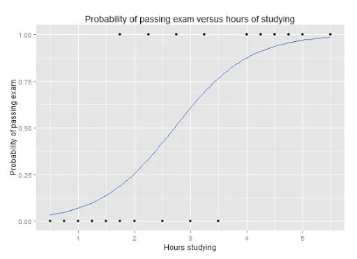
[Figure 2]
This is not just restricted to data science and finds application in statistical applications like multivariate analysis.
3. Decision Trees
A decision tree is a decision support model that is often represented as a tree-like visual and shows the decisions and possible outcomes. It allows organizations to either lead informal discussions or map out an algorithm that predicts the best decisions mathematically. It is a flow-like structure where each internal node represents a test, each branch represents an outcome, and each leaf is a class label. The path of going from the top to the bottom represents all of the classification rules.
Used frequently in classification problems, decision trees are simple to understand, interpret, and visualize. They usually require little effort for data preparation and are highly used in supervised learning algorithms.
[Figure 3]
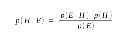
4. Naive Bayes
Naive Bayes models are perfect for solving text classification problems. This model assumes all variables are independent. Naive Bayes is used to calculate the probability that an event will occur based on those that have already occurred while assuming both events are independent of each other.
In short, it is a probabilistic classifier. A great example is using this model to try and classify spam emails. Using a training dataset, a user can teach the model to identify keywords and phrases which show up on previous spam emails and calculate the probability that a new email is a spam, then classify it accordingly.
As in the name, this model uses the Bayes Theorem of Probability
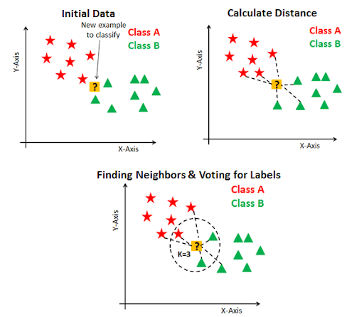
5. K Nearest Neighbor (KNN)
Unlike other machine learning models, KNN uses the entire dataset rather than splitting into training and production sets (Here's the perfect parcel of information to learn data science). A type of supervised learning, KNN can make predictions for new data points by searching the entire dataset for the “K” most similar occurrences (nearest neighbors) and returning the output value for those K instances.
You may also like: Tips to ace your Data Science Interview
In order to determine which of the K instances the new data point is most similar to, a distance measure is used. The most popular distance measure for this model is Euclidean distance.
[Figure 4]
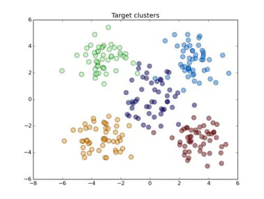
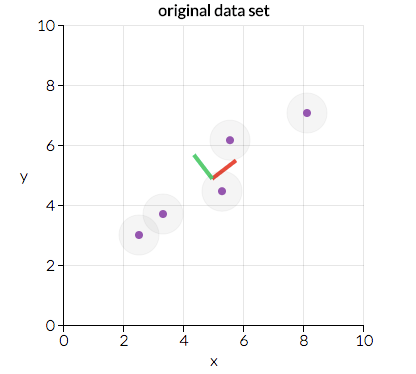
6. K Means Clustering
K Means is one of the most popular clustering algorithms used in machine learning. It is an excellent model to use when trying to categorize unlabeled data together, into clusters, based on certain features and their values. It groups the data together with the number of groups represented as the variable K. The model then runs through iterations assigning each data point to one of the defined K groups. Finally all the data points are clustered together based on feature similarity. A common use case of K Means is segmenting customers into groups to better predict who could be a returning customer, or who might be willing to take a survey.
[Figure 5]
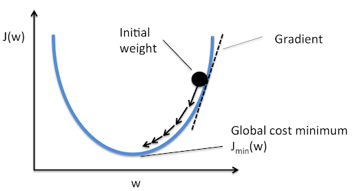
7. Gradient Descent
The gradient descent model is best used when seeking to minimize a certain function, often described as a minimum cost function.
Imagine if you were trekking down from a mountain that you were unfamiliar with, and your goal was to get down as fast as possible.
Of all the possible directions you could go, the gradient descent model would use the path that results in the steepest descent, while also considering the paths that take less time.
As you move down the mountain you’re able to better predict each new step and path. Repeating the process of trekking down the mountain enough times will eventually lead to the bottom, thus exposing the values of the coefficients that result in the minimum cost.
[Figure 6]
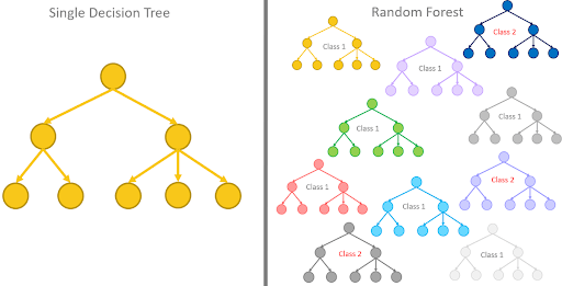
8. Random Forests
The underlying model within a random forest is a series of decision trees. The decision trees are only able to predict to a certain degree of accuracy.
But when combined together, they become a significantly more robust prediction tool. Random Forests run efficiently on large data sets and train each tree with a random sample of data points. The model comes to a final prediction by averaging the outcomes of each individual decision tree.

[Figure 7]
9. PCA (Principal Component Analysis)
The main objective of a principal component analysis is to reduce the dimensionality of a dataset where a lot of variables exist. When working with a lot of variables it can be challenging figuring out which ones directly relate to each other and to a prediction.
In order to find which variables you need to focus on, the principal component analysis uses feature elimination or feature extraction to reduce the dimensionality. Feature extractions provide better results as they allow the model to create “new” independent variables that are a combination of the existing variables.
You may also like: How to Become a Data Scientist in 2020
In essence, the model transforms the existing variables into a new set of variables which are known as the principal components.
This model is excellent to use when presented with a large dataset with lots of variables and performing exploratory data analyses.
[Figure 8]
10. XGBoost
One of the more recent popular models dominating headlines has been the XGBoost algorithm. Essentially it is an implementation of gradient boosted decision trees that are designed for speed and performance.
XGBoost stands for eXtreme Gradient Boosting. It has been made available in a software library that anyone can download and install.
The two main reasons to use XGBoost happens to also be the two goals of the model itself.
1. Execution speed
2. Model performance.
Because of those goals, it has risen to be the go-to model for many machine learning specialists and is a great model to have in your toolkit.
Wrap Up
The most common question a beginner may ask when facing a variety of machine learning models is, “which one should I use”? The answer depends on a few factors, such as the quality and size of your dataset and the urgency of the request, but ultimately what question are you trying to answer? Even the most experienced data analysts and scientists try a few different models before finding the right one. As you continue to learn about machine learning and understand more models, you will begin to grasp the strengths and weaknesses of each model.