Hey Alexa, play some music!
Hey Alexa, what is the cricket score today?
Have you ever had interactions like these?
If so, as a user, you have pretty much explored artificial intelligence at length!
Deep learning, commonly known as a neural network, is the approach that artificial intelligence (AI) uses. The concept of artificial intelligence was originally proposed in 1944 by two researchers, Warren McCullough and Walter Pitts, from the University of Chicago, USA.
You may also like: How to Drive Business Value with Robotic Process Automation(RPA)?
What Is A Neural Network?
Have you ever thought about what a neural network is?
The word ‘neural’ comes from neurons and the network suggests a connection between those neurons.
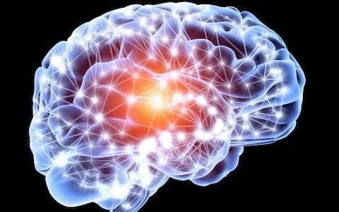
Source: telegraph.co.uk
The neural network in AI is based on the concept of biological neural networks. In general, our brain is connected with more than 80 billion neurons (Source). The human neural system has three stages: receptors (receive the stimuli and pass the information to the outside environment), neural networks (make a decision for output after processing the input), and effectors (translate information of neural networks into a response) (Source).
Source: neurosciencenews.com
The concept of deep learning is also based on a similar approach. We will see the whole concept of neural networking of AI using the Artificial Neural Network (ANN).
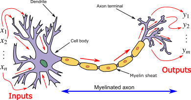
Source: en.wikipedia.org
Application of Deep Learning
Deep learning has altered our world and its application is widely used in many fields such as image classification, speech recognition, language transition, sentiment analysis, cancer cell detection, diabetic grading, drug discovery, video search, face detection, video surveillance, satellite imagery, pedestrian detection, lane tracking, and recognition traffic signs. These are only a few examples of deep learning. This field is now beyond imagination.
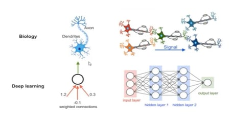
Here is a look at the structural similarity between a neuron and the weighing function that have pathways towards and away from the cell body or node.
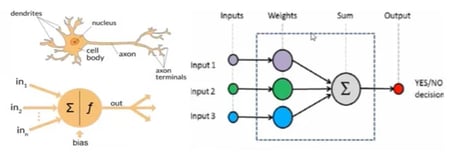
In the same way, here is the biological structure of neurons that are connected with each other via synapses across which signals are passed
Important Concepts Used In Artificial Neural Network (ANN)
Before moving ahead, let’s discuss some important concepts used in ANN.
- Perceptron
A perceptron is known as a single neuron model that is the basic building block to larger neural networks.
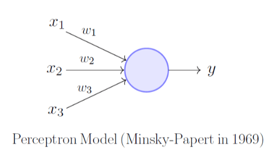
In this example, the perceptron has three inputs x1, x2, and x3 and one output. Weights (w1, w2, and w3) define the importance of these inputs. The output here is 0 or 1 as used in the classification model.
Output = w1x1 + w2x2 + w3x3
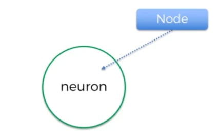
- Neurons
Neurons or nodes are the base of neural networks. The concept of neurons is derived from biological neurons.
Each neuron may have one or many inputs. Likewise, one neuron may yield single or multiple outputs to multiple neurons.
- Synapse
ANN is made up of connections. These connections are more commonly known as weights or synapse. Each synapse in ANN is the output of one neuron and input for another connection layer neuron. Weights have an important role, as they are used for a neural network to learn. Weights are supposed to adjust or pass the signal to the next neurons.
All of these weighted values summed up in relevant neurons and then activation function is applied to the weighted sum. Based on the activated function neurons will either pass the signal or not. Activation functions play a pivotal role in firing the ANN. There are many types of activation function, however, threshold function, sigmoid, rectifier, and hyperbolic tangent are the most common ones. The explanation of these activation functions is beyond the scope of the current blog. Hence, readers are suggested to explore more about these activation functions.
Source: neuralnetworksanddeeplearning.com
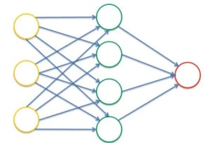
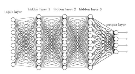
- Hidden layer
The hidden layer is a layer of neuron in ANN which is present between the input and output layer. The input layer receives the data. The weighted sum of the input layers then transfers to the first hidden layer using the activation function. ANN may have a single hidden layer, no hidden layer, or multiple hidden layers.
- Hyperparameter
To run ANN, several constant parameters are set before the learning process begins. Some examples of hyperparameters are a number of hidden layers, epoch, batch size, optimization, etc. All of these are explained in the relevant section.
- Forward propagation
In this step, the neural network is fired in the forward direction, from left to right. Input layers move to the next hidden layer based on weight and this step moves forward as per the activation function, until getting the predicted results y.
.png?width=365&height=80&name=ann%20fp%20(1).png)
Source: neuralnetworksanddeeplearning.com
- Cost Function
Cost function and loss function refers to nearly the same thing. It basically compares the predicted results to the actual result and measures the generated error.
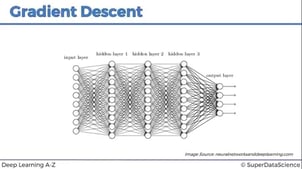
- Backward Propagation
As suggested, backward propagation moves from right to left. This is an algorithm that uses gradient descent to calculate the gradients of the error function. The most commonly used gradient descent is stochastic gradient descent. The explanation of gradient descent is beyond the scope of this blog. Hence, readers are suggested to explore more information about gradient descent. This step is back-propagating the error. Weights are updated based on the error. The learning rate depends on the weight update.
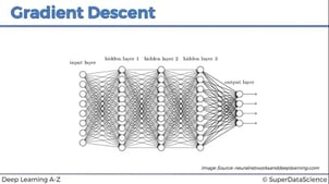
Source: neuralnetworksanddeeplearning.com
How to Perform An Artificial Neural Network Step-by-step?
Now it is time to perform the ANN. However, there are many platforms for python that can be used to perform machine learning. Here, Google Colab is used since no library installation is required. You just need a Gmail account.
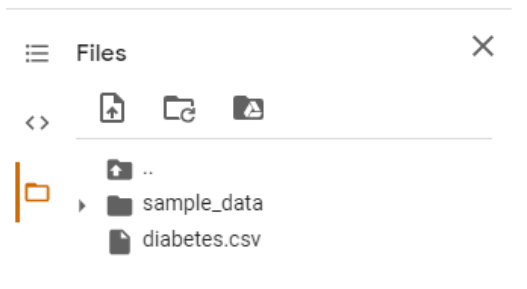
Step 1: Upload Dataset
Step 1 of any data analysis in Google Colab is to upload the data set. Here, the Pima Indian diabetes dataset is uploaded first.
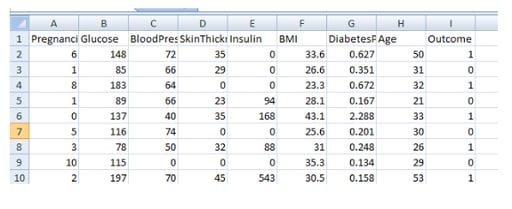
This dataset is available on Kaggle (link). The diabetes dataset contains several columns that may play an important role in the risk of diabetes. These columns are:
- Number of pregnancies
- Glucose
- Blood pressure
- Skin thickness
- Insulin
- BMI
- Diabetes pedigree function
- Age
- Outcome (diabetic or non-diabetic)
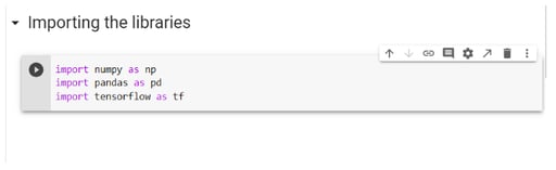
Step 2: Importing The Libraries
Libraries in python play a pivotal role in data analysis. Here, NumPy, pandas, and TensorFlow have been imported. It is important to remember that you may face different types of challenges in different datasets. Hence, you may have to use a different set of libraries or many other libraries.
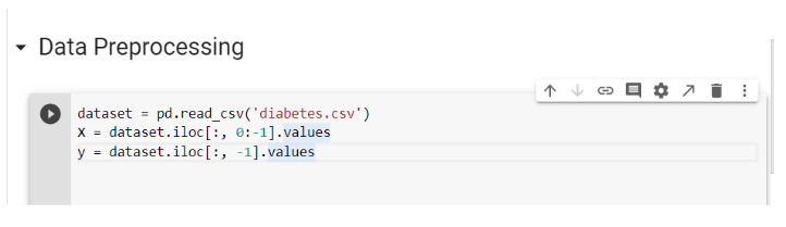
Step 3: Data Preprocessing
It is difficult to imagine any data analysis with the preprocessing of the data set. Again, every dataset comes with a different challenge. Hence, excellent knowledge of python is essential. The most common challenge in data preprocessing is the exclusion of inconsequential columns and conversion of categorical data, such as gender into 0 and 1. The current diabetes dataset only requires separation of independent (X) and dependent (y) variables. Pandas library was used to read the dataset and the formation of dependent and independent variables.
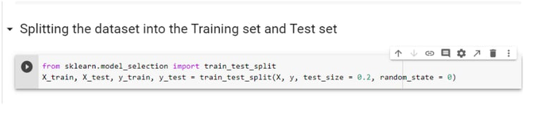
Step 4: Splitting the Dataset into the Training set and Test set
Splitting of the dataset into training and test sets is necessary. The training set is used to apply the machine learning model. Hence, a large portion of data is randomly selected as a training set from the whole dataset. Here, 80% of data is selected as a training set (test_size = 0.2). The random state is required to achieve a similar splitting of dataset each time we run ANN. Otherwise, there will be a slight change in results. The test set is used to evaluate the model. Scikit library is required to split the dataset.
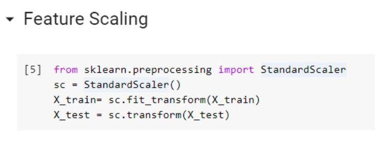
Step 5: Feature Scaling
The most frequent question asked in machine learning is when to use feature scaling (before splitting the dataset or after splitting the dataset)?
You must get a clue that it should be done after splitting the dataset into training and test sets. Feature scaling is performed to normalize or standardized all independent variables. Some variables, such as age and salary are totally on different scales, hence may have a different effect on Euclidean distance (there are many other ways to calculate distance such as Manhattan distance). Therefore, all independent variables should be on the same scale. If we perform feature scaling before splitting the dataset, the mean value of the whole data set will influence the result. Hence, feature scaling should be done after scaling the data set. Feature scaling is an essential step as there is going to be a lot of computation in ANN and you wouldn’t want any independent variable to dominate on any other variable.
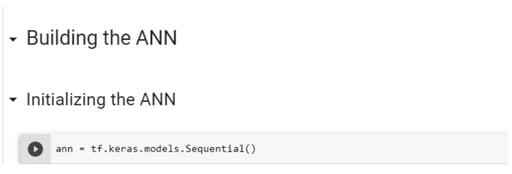
Step 6: Building the ANN model
The next step of ANN is to build a model.
Step 6.1: Initializing the ANN
Earlier you were loading Tensorflow and Keras separately to create a sequential model. Keras library is now integrated into the new version of TensorFlow (2.0). Sequential class is used to initialize the ANN as a sequence of layers.
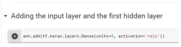
Step 6.2: Adding the Input Layer and the First Hidden Layer
The next few steps required the formation of sequence layers for ANN. In this step, you will be adding the input layer and the hidden layer. To add these layers, you should use a dense class. This dense class is used in whatever phase of the neural network we are, as it is also evident by my few next steps. Here, the add method is used to add anything such as a hidden layer from the sequential class using the ‘ann’ variable created in the previous step. The layer module is used to add classes, which means layers you want to add in our ANN. The number of units here suggests a number of hidden neurons or hidden layers. Our input neurons or layers are all of our independent variables.


You may also like: 10 Machine Learning Models to Know for Beginners
The next most important question in ANN is how many hidden layers you want?
Is there any specific rule or it should be based on trial and error. There is no specific rule to choose a number of units. It is experimentally based. You have to use different hyperparameters. Here, you can see four, based on several trials. There are many functions that may require based on different approaches. In this blog, you will see just two of the unit and activation functions. For a fully connected hidden layer, the rectifier activation function (relu) is used. This rectifier function is mostly suggested to connect hidden layers. Nonetheless, it is good to have a basic understanding of all activation functions, as things may change based on different datasets.
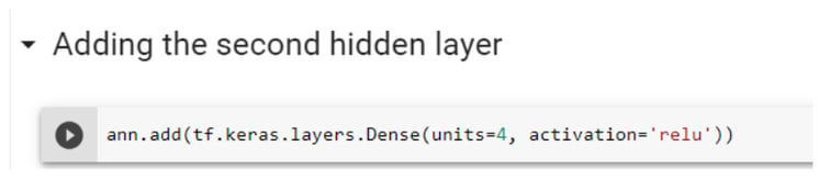
Step 6.3: Adding the Second Hidden Layer
The next step is adding the second hidden layer. All required steps given below are explained above (step 6.2).
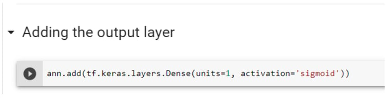
Step 6.4: Adding the output layer
Adding the output layer in ANN is slightly different than adding a hidden layer. It is important to know the dimension of the output layer. In this dataset, you will be predicting binary variables (0 or 1), hence dimension is one. It means you just need one neuron to predict the final output. Remember, this is an example of a classification approach. Another important change in this layer is the activation function. Here, you can see the use of the sigmoid function, because it not only gives a better prediction than rectifier function but also provide the probabilities. Hence, you will get the prediction that if someone is having diabetes or not, including their probabilities.
Now all layers required for ANN are ready.
Step 7: Training the ANN
The next step is to train the created model on our training set. Training of ANN requires two steps.
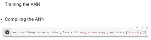
Step 7.1: Compiling the ANN
The first step is to compile the ANN with an optimizer, lost function, and metrics. Here, in metrics, you are using accuracy function, as you are using classification (binary dependent variables). The first argument is the optimizer. The optimizer is used for the optimization algorithm we want to use to find the optimal set of weights in the neural networks. Here, you will be using ‘adam’ optimization which is an extension of stochastic gradient descent. If you check the mathematical detail of stochastic gradient descent, you can find that it is based on the lost function that you need to optimize to find the optimal weights. The lost function is not the sum of squares square errors like for linear regression but it's going to be a logarithmic function that is called a logarithmic loss. When the weights are updated after each observation or after each batch of many observations the algorithm uses this accuracy criterion to improve the model’s performance. The name adam is derived from adaptive moment estimation. Next is computing the cross-entropy loss between true labels and predicted labels. Use this cross-entropy loss when there are only two label classes (assumed to be 0 and 1).
Step 7.2: Training the ANN on the Training set
The next step is fitting the ANN of the training dataset. Two arguments in this example are used to fit the training model, epochs, and batch size. The sample size for the diabetes dataset is 768. Batch size 50 suggests the number of samples processed before our ANN model is updated. One epoch is when an entire dataset is passed forward and backward through the neural network only ONCE.
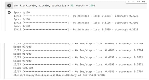
This step may take time based on given arguments and the size of the data.
Step 8: Making the Predictions and Evaluating the Model
Now the ANN model is ready and also performed on the training dataset. But, how would we know if it is good? We will check our model using the test data set, however, only using independent variables. Results from the predicted test dataset will then be compared with the original results.
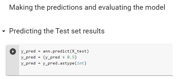
Step 8.1: Predicting the Test set results
As the dataset being used has a binary outcome, a classification approach of supervised machine learning is used here. The first step is to predict the outcome of the test dataset using the independent variable, here X_test, using the ‘ann’ model trained on the training dataset. As you used sigmoid activation function for output, hence the results are in probability. Next, you will have to convert those probabilities into true ( > 0.05) or false (<0.05) and then change those true and false into 0 and 1.
Step 8.2: Making the Confusion Matrix
The confusion matrix is used to compare the predicted results of the test dataset with the original results of the test dataset. Scikit library is required to create a confusion matrix, here 2 x 2 table.
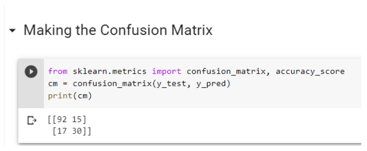
Result:
True positive: 92 (Diabetic)
True negative: 30 (non-diabetic)
False-positive: 15 (Non-diabetic but predicted as diabetic)
False-negative: 17 (diabetic but predicted as non-diabetic)
Step 10: Calculate the Accuracy score
Accuracy calculation also requires the Scikit library. It shows how good the model is.
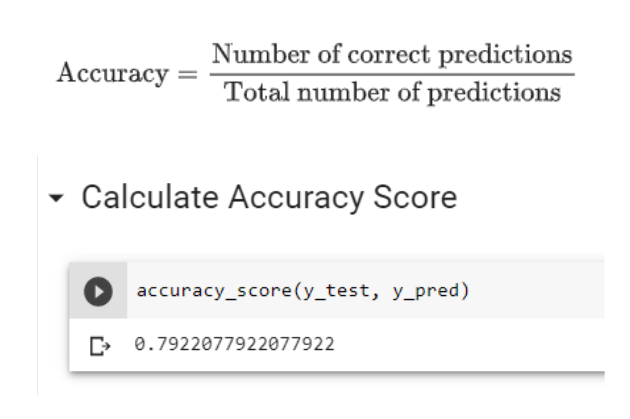
The accuracy of the model prediction is 79.22%. Actually, it is a good prediction. It is impossible to get 100% accuracy. If you get 100% accuracy for your model, then think again. That model is too good to be true. Hence, the rechecking of those models is highly recommended.
In this blog, you will find an explanation of common terminologies used in ANN. However, readers are suggested to explore more information about neural networks and ANN. Remember each dataset is different; hence you may have to use different approaches, including hyperparameters more suitable for that dataset. Start your journey in ANN today and deep dive as much as possible.
We offer an instructor-led Data Science Course. Click here to learn more!