Linear Regression With Python scikit Learn

Regression is a way of assessing the relationship between possible causes and observed effects.

It finds use in different domains from Economics to Healthcare to Science to ascertain the relationship between the independent (cause) variables and dependent (effects) variables.

In this modeling technique, a set of statistical processes are used for estimating the relationships among variables. 

Types of regression techniques

1. Linear Regression

a. Simple Linear

b. Multiple Linear

2. Logistic Regression

3. Polynomial Regression

4. Stepwise Regression

a. Forward Regression

b. Backward Regression

5. Ridge Regression

6. Lasso Regression

What is a Linear Regression?

Of all the handy ML models out there, linear regression is a common, simple predictive analysis algorithm. It is applicable when the dependent variable is continuous in nature. This is a supervised machine learning algorithm.

This algorithm tries to estimate the values of the coefficients of the variables present in the dataset (also consider checking out this perfect parcel of information for a data science degree). The coefficients determine the strength of the correlation.

It attempts to make a model that gives the relationship between two variables by applying a linear equation to observed data.

Assumptions/Condition for Linear Regression:

1. Linearity: The relationship between the independent variable and the mean of the dependent variable is linear.

2. Homoscedasticity: The variance of residual is the same for any value of the independent variable.

3. Independence: Observations are independent of each other.

4. Normality: For any fixed value of the dependent variable, the dependent variable is normally distributed.

What is Simple Linear Regression?

Simple linear regression is a type of regression that gives the relationships between two continuous (quantitative) variables: One variable (denoted by x) is considered as an independent, predictor, or explanatory variable. Another variable (denoted by y) is considered as a dependent, response, or outcome variable.

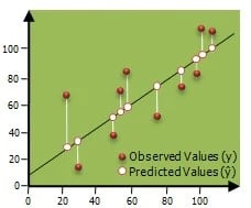
In the figure below, we can see that we have two variables x and y which have some scattered. Through the scatter plot, there is a line passing through. This called a Regression line or the best fit line.

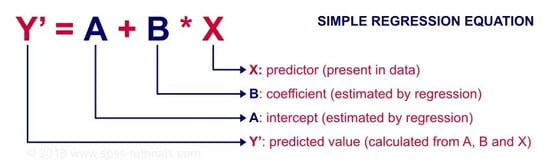
The math behind the best fit line:

Use the following steps to find the equation of the line of best fit for a set of ordered pairs (x1,y1),(x2,y2),...(xn,yn)

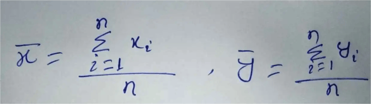
Step 1: Calculate the mean of the x-values and the mean of the y-values.

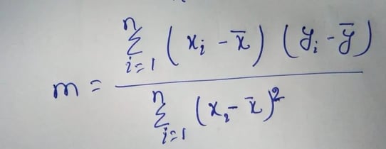
Step 2: The following formula gives the slope of the line of best fit:

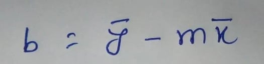
Step 3: Compute the y-intercept of the line by using the formula:

Step 4: Use the slope m and the y-intercept b to form the equation of the line.

Some important topics related to Regression

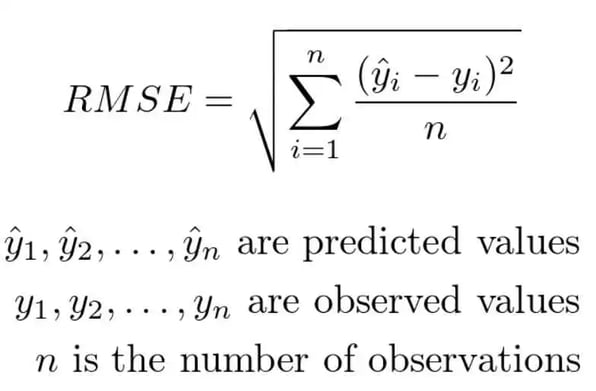
RMSE:

It stands for Root Mean Square Error.  It equates to the square root of the squares of the sum of differences between each observed data value and the predicted value. The minimum value of the RMSE is the best for the best fit line. Basically, it is the square root of variance.

In other words, it is the standard deviation of the predicted values. It is a parameter to measure the distance between the data point and the regression line. It measures how spread out these residuals are. In simple words, we can say that it tells us how distributed the data is around the line of best fit (also consider checking out this career guide for data science jobs).

R-squared (R²):

It measures the proportion of the variation in our dependent variable vis-a-vis the independent variables in the model.

It assumes that every independent variable in the model helps to explain variation in the dependent variable. In reality, some independent variables (predictors) don't help to explain the dependent (target) variable.

In other words, some variables do not contribute to predicting the target variable.

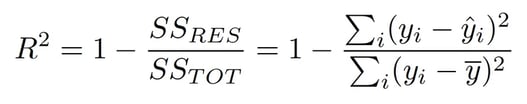
Mathematically, we can calculate it by dividing the sum of squares of residuals (SSres) by the total sum of squares (SStot) and then subtract it from 1.

In this case, SStot measures the total variation. Ssreg measures explained variation and SSres measures the unexplained variation.

As SSres + SSreg = SStot,

R² = Explained variation / Total Variation

R-Squared is also called the coefficient of determination. It lies between 0% and 100%. 

An r-squared value of 100% means the model explains all the variation of the target variable. And a value of 0% measures zero predictive power of the model. 

So, the higher the R-squared value, the better the model.

Adjusted R-Squared:

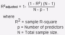
The Adjusted R-Squared measures the proportion of variation explained by only those independent variables that really help in explaining the dependent variable.

It penalizes us for adding an independent variable that does not help in predicting the dependent variable.

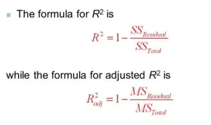
Mathematically we can write it in the following manner:

Difference between R-squared and adjusted R-square:

1. Adjusted R-square can be negative only when R-square is very close to zero.

2. Adjusted R-Square values are always less than or equal to R-square but never be greater than R-Square.

3. If we add an independent variable to a model every time then, the R-squared increases, despite the independent variable being insignificant. This means that the R-square value increases when an independent variable is added despite its significance. Adjusted R-squared increases only when the independent variable is significant and affects the dependent variable.

Multicollinearity:

It occurs when one or more independent variables are correlated with one or more independent variables. This problem arises in Multilinear Regression where two or more independent variables are involved in the regression. Multicollinearity only affects variables that are highly correlated.

There are two popular ways to find multicollinearity:

1. To compute a coefficient of multiple determination for each independent variable.

2. To compute a variance inflation factor (VIF) for each independent variable.

With the concepts clear, let us move on to the implementation. I suggest you do this side-by-side with the tutorial.

Implementing Linear Regression In Python - Step by Step Guide

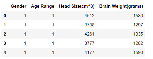
I have taken a dataset that contains a total of four variables but we are going to work on two variables. I will apply the regression based on the mathematics of the Regression.

Let’s start the coding from scratch.

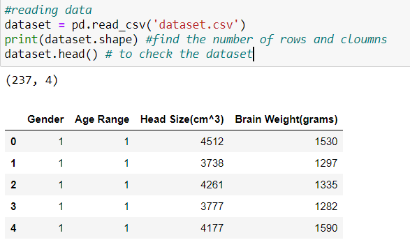
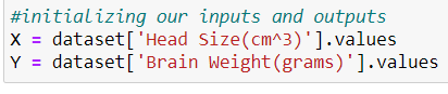
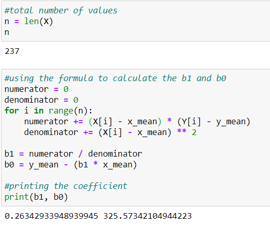
For this example, we will work on with the Head Size(cm^3) and Brain Weight(grams), initializing them as X and Y, respectively. 

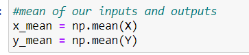
Now let's calculate the mean of the X variable and Y variable.

In the figure below, we can see the coefficients b1 and b0 for the regression line. Here b0 is the y-intercept, and b1 is the slope.

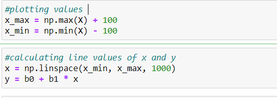
Next, we check the regression line with the data points.

In this plot, we can see the data points are in the form of green dots, and the regression line is in red color.

On the x-axis, we kept Head Size, and on the y-axis, we kept Brain weight.

Here is the code to assign these labels:

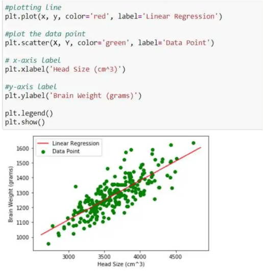
From the above figure, we have to recall the assumptions of linear regression (data should be linear scattered), and this can be seen in the graph.

Now let's work on the RMSEE values and try to find the best fit line.

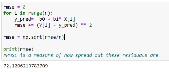
Here we can see the formula of RMSE once again.

Now we have to find the accuracy that will show whether our model is good or not.

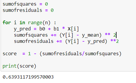
With our accuracy at 63.93 %. there is some room for improvement. 

We do this by directly using Sklearn and statistics libraries in the python.

Implementation of Regression with the Sklearn Library

Sklearn stands for Scikit-learn. It is one of the many useful free machine learning libraries in python that consists of a comprehensive set of machine learning algorithm implementations.

It is installed by ‘pip install scikit-learn‘.

So let's get started.

For this linear regression, we have to import Sklearn and through Sklearn we have to call Linear Regression.

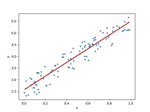
Before we implement the algorithm, we need to check if our scatter plot allows for a possible linear regression first.

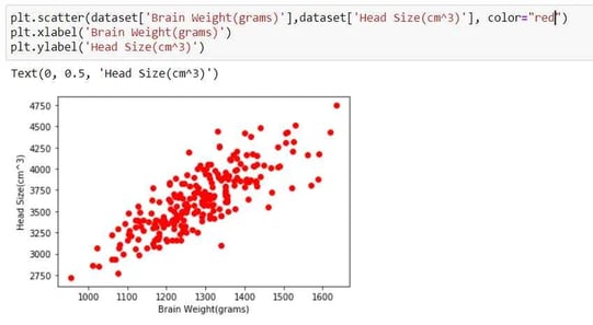
From the above plot, we can see that our data is a linear scatter, so we can go ahead and apply linear regression to our dataset.

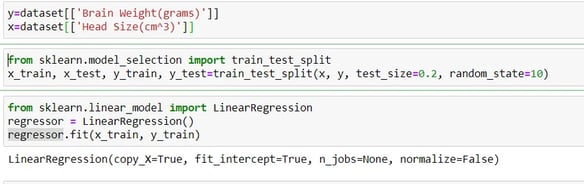
First, I have divided our dataset into dependent and independent variables, like in x and y. 

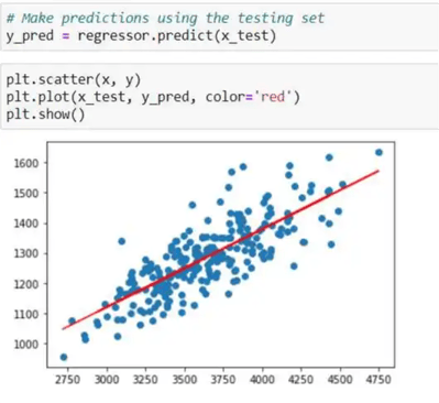
Next, I have applied a train test split from the Sklearn library. This is so that we can divide our dataset into a training set and a testing set (Remember we said that this was a Supervised machine learning algorithm?) with a test size of 20%.

In the next cell, we just call linear regression from the Sklearn library. And try to make a model name "regressor". In the next line, we have applied regressor.fit because this is our trained dataset.

Now, let’s check the accuracy of the model with this dataset.

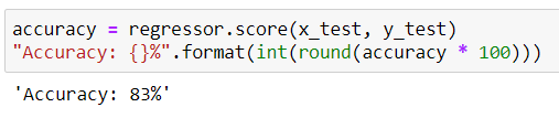
Again, I tried to check the regression line in our dataset.