5 Hidden Tricks In Microsoft Excel You Must Know

These 5 best tricks in Microsoft Excel are probably unknown to you. Remember, they possess the marvelous abilities of making you an expert in handling the databases saved on spreadsheets. Find out how!

Are you an industry expert with high analytical skills? Probably, you are also a regular user of Microsoft Excel.One thing is for sure; if these tricks and shortcuts are unknown to you, simple spreadsheet tasks mayappear to be lengthy and hectic processes that will make you sweat. Here, we bring forth a few of the best hidden tricks that may benot known to you. 

1.Make a Reusable Chart Template

Say, you are at the end of a financial year and your boss has asked you to present your company’s annual report within a short time period. We all know that creating an annual report would indicate making a series of charts, all engraved in the same format. Here is the trick that will allow you to go about this task faster than ever. 

• The first step would be to create a chart and format it in just the way you want the series of charts to look.

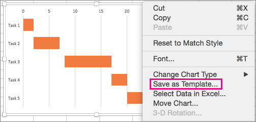
• For saving this format as a template (excluding the data), select Chart Tools, then Design Tab. 

• After this, select Save as Template and then give a name to the final output.

 

• For using this template to make a new chart, start by selecting the data. 

• Use Ribbon Toolbar for this. 

• Select Insert, then Other Charts and finally All Chart Types. 

• Next, you will have to click on the Templates option. 

• From My Template Group, choose the template that you have already saved and then click on OK. 

Bingo, the new chart will have the same style as the template chart. Thus the time tha could have gone in formatting charts repeatedly is saved!

2. Dealing with Large Data Volumes with Watch Window

Assume that you are working on the calculation of ‘10 years’ employee benefits’ data. It seldom happens that you need to see the entire set of changes that take place in the worksheet when you change a figure in any particular area. However, how do you see the changes in the areas that are sitting off-screen? You can do so by setting up a Watch Window!

For the watch window:

• Left click the mouse on the cell that you want to see.

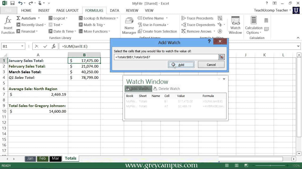
• From the Ribbon toolbar, select Formulas and then Watch Window. 

• As the dialog box appears, click on Add Watch. 

• Since you have already selected the cell, just click. 

• Add after confirming the cell number. 

Now, go to the area which you were editing; you will find the Watch Window floating at the top of your worksheet. As you edit, the Watch Window will keep on displaying the changes in other cells. 

Move and resize the Watch Window is as per your wish. You can use the Add Watch option for seeing additional cells within the Watch Window. You can also view cells that are present in other worksheets.

3. Making Formulas Easy to Understand

In general, an excel spreadsheet would show up the formulas with the cell number, say, “=B5*C6”. No doubt a formula that looks like, say, “=DailyWage*C6” is much easier to interpret and understand. You can create formulas that look like the latter if you assign common names to the cells that contain repeatedly used data. 

• For naming a range, firstly, you need to click on the particular cell or select the cell range that you want to name. 

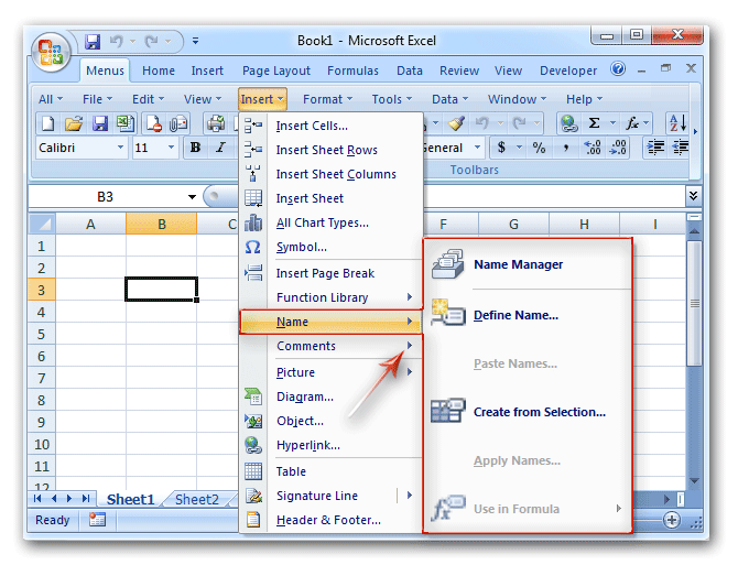
• From the Ribbon Toolbar, select Formulas, then Define Name; next, you type the required name in the Name box. 

• Click on OK.

 

 When you name the cells on an Excel sheet, you get the privilege of finding any of the cells or ranges by just clicking on the Name Box. By clicking on the drop down arrow given there, you can see the list of all the named cell ranges. Click on any name to go to that particular area on the sheet right away.

4. Printing a Number of Sheets on a Single Page

It is impossible for any built-in command or option to produce a printed page that is composed of data from a number of sheets in a particular workbook. Well, you have a way out for this too; it involves the use of the popular Camera tool. 

• To begin with, add the Camera icon to the toolbar, the simplest way is to use the Quick Access Toolbar.

• Click on the drop pointing arrow on the right of Quick Access Toolbar and select More Commands. 

• You can find a drop down list in the dialog box that appears. 

• There, you choose Commands Not in the Ribbon and then click on the Camera icon.

• Select ‘Add’ to place it on the Quick Access Toolbar. 

• Then click on Close!

The next step would be to select the first range that you want to print. Take a snapshot by clicking on the Camera icon. 

• Go to a new sheet and click over the cell where the snapshot should appear.

• As soon as you click, the snapshot image would appear there. 

• Then, you go to the second range that is to be printed. 

• Take the snapshot and repeat the same process as before.

• Assemble all the data on the worksheet and take the print out.

The best part is that if you change any of the cells in the original data, the snapshots’ data changes automatically.

5. Making a List of Custom Data–Entry

Typing the same data time and again is a tedious task when you have lots of other important assignments to accomplish. Microsoft Excel has a hidden trick that allows you to choose the data entry from an already prepared list. So, if you are working on an appraisal sheet of the same number of employees for the past five years or so, set the list up in that way. 

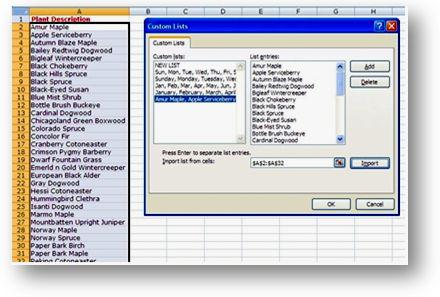
• For creating such a custom list, you need to type the list in a single column in an empty sheet.

• Now, come to the sheet where you want to use this list. 

• Next, select the range where you need the list to be entered. 

• Select Data, then Data Validation and finally the Settings Tab. 

• Select list within the Allow drop down menu. 

• Then, you need to click on the Source area, go to the sheet where you have typed the data, and then select the data. 

• Click on OK for closing the dialog box. 

When any such cells are selected (to which the Data Validation option has just been activated), you will find a drop-down arrow. On clicking the arrow, you will find a list of items that can be selected to be pasted in the cell.

Way Forward

So, are you all set to take up the new challenges in your work field? Use these truly usefulhidden tricks of Microsoft Excel for preventing the wastage of time and money. You will be relieved to know that working with spreadsheets is not so hectic now!